Determine Heat Generation in Plastic Deformation | Ansys Mechanical WB
Relationship between Heat Production, Plastic Deformation, and Stress Level
Ansys Mechanical APDL has multiphysics element types that can use displacement and temperature degrees of freedom at their nodes, support nonlinear structural and thermal material properties. In addition, allowing engineers to understand and predict heat generation in plastic deformation.
This permits modeling of thermoplastic heat generation with Ansys Multiphysics and with Ansys Mechanical licenses.
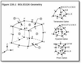
This article uses the SOLID226 20-node brick high order element in such an application. Note the importance of the correct units for Specific Heat, Thermal Conductivity and Thermal Loads in models of this type.
Selection of an Element to Support Thermoplastic Heat Generation
Three Ansys elements support the thermoplastic effect, “which manifests itself as an increase in temperature during plastic deformation due to the conversion of some of the plastic work into heat” (Theory Reference, 11. Coupling, 11.3. Thermoplasticity). Thermoplastic analysis exists in the following Ansys elements:
PLANE223 – 2-D 8-Node Coupled-Field Solid
SOLID226 – 3-D 20-Node Coupled-Field Solid
SOLID227 – 3-D 10-Node Coupled-Field Solid
Setting KEYOPT(1) to 11 activates displacement and temperature degrees of freedom for these elements.
During direct coupled analysis, structural-thermal coupling can have Strong (matrix) coupling which produces an unsymmetric matrix, or Weak (load vector) coupling which produces a symmetric matrix and requires at least two iterations per substep. Coupling choice is set with KEYOPT(2). As quoted below, Weak coupling is recommended in static and transient analysis. The Coupled-Field Analysis Guide, 2. Direct Coupled-Field Analysis mentions Strong coupling if contact elements are used. Note the following comments:
“Because of the possible extreme nonlinear behavior of weakly coupled field elements, you may need to use the predictor and line search options to achieve convergence.”
“To speed up convergence in a coupled-field transient analysis, you can disable the time integration effects for any DOFs that are not a concern. For example, if structural inertial and damping effects can be ignored in a thermal-structural transient analysis, you can issue TIMINT,OFF,STRUC to turn off the time integration effects for the structural degrees of freedom.”
In the Coupled-Field Analysis Guide, 2. Direct Coupled-Field Analysis, 2.6. Structural-Thermal Analysis it states:
“In a structural-thermal analysis with structural nonlinearities using elements PLANE223, SOLID226, and SOLID227, it is recommended that you use weak (load vector) coupling between the structural and thermal degrees of freedom (KEYOPT(2) = 1) and suppress the thermoelastic damping in a transient analysis (KEYOPT(9) = 1). When using the SOLID226 element, you should also select the uniform reduced integration option (KEYOPT(6) = 1). These options will be automatically set if ETCONTROL is active.
“PLANE223, SOLID226, and SOLID227 also support a thermoplastic effect calculation in static or transient analyses. For more information, see Thermoplasticity in the Mechanical APDL Theory Reference.”
In the present example, the above recommendations have been considered.
In more general 3D meshing, users will want to consider the use of both the SOLID226 and SOLID227 elements for this sort of coupled analysis.
For further reading, users can consult: Theory Reference, 11. Coupling, 11.3. Thermoplasticity
Materials for Thermoplastic Heat Generation
In addition to the usual thermal and structural material properties, elements that capture Thermoplastic Heat Generation will require the Taylor-Quinney coefficient (input as QRATE on the MP command) which is the decimal fraction of plastic work that is converted to heat, and a model of material plasticity, such as Isotropic or Kinematic Hardening. Typical QRATE values might fall in the range of between 0.80 and 0.95, however, users will be responsible for finding values that are appropriate for the materials being studied. Required material properties will include MP commands for structural and thermal behavior. An example in SI units for a fictitious steel material is:
Youngs Modulus of Elasticity EX=0.2070000E+12 MPa
Poisson’s Ratio NUXY=0.2900000
Coefficient of Thermal Expansion ALPX=0.1510000E-04
Density DENS=7850.000 kg/m3
Thermal Conductivity KXX=46.70000 W/m/C
Specific Heat C=419.0000 W/kg/C
Taylor-Quinney Coefficient QRATE=0.9000000
Heating due to plastic deformation will require a material plasticity model input with TB commands. A simple example in SI units is a Bilinear Isotropic Hardening model with:
Yield Stress 1.0e8 MPa
Tangent Modulus 1.0e9 MPa
If heat is to be produced, loading high enough to cause yielding and plastic deformation will be required.
UNITS in the Model
Proper use of Units in the model must be emphasized. Thermal loads must be in appropriate energy units. Plastic strain energy will be in the units of Force × Distance. Material properties for Thermal Conductivity and Specific Heat must contain energy expressed in the form of this physical work, not units such as BTUs in US Customary units. It is simplest to do everything in SI units, as employed in the present example. Note the units of Watts (Joules per second, i.e. Newton-Meters per second) above.
Users desiring to work in units such as inches or millimeters must represent Thermal Conductivity and Specific Heat in energy units in inch-pounds for the inches system, or millimeter-Newtons for the millimeters system, respectively. This type of conversion is hidden from the user but is employed internally when Workbench Mechanical is chosen for thermal analysis.
Loading on the Model
The model has symmetry constraints on the back, left, and bottom sides. The right-hand side has a non-zero displacement in the +X direction—enough to cause 10% total strain in the model X direction. The solution has been set up to ramp up the non-zero displacement through many Substeps in one Load Step.
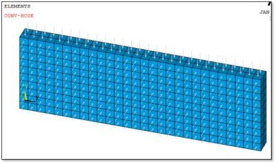
The model has a convective heat transfer surface load on the top and front sides. In the following Figure 4, grey arrows show where the convective load is applied. The arrows are grey because a Table Array that is a function of Time is used to apply a constant convective load that does not vary over time during substeps.
Some users consider adiabatic loading, with the assumption that the deformation event is so rapid that there is no significant conduction of heat. This can be mimicked in Ansys with a short time interval. The adiabatic effect can also be suggested if thermal loads are removed, and a near-zero thermal conductivity is entered. Users need to consider whether near zero thermal conductivity creates thermal transient analysis difficulties.
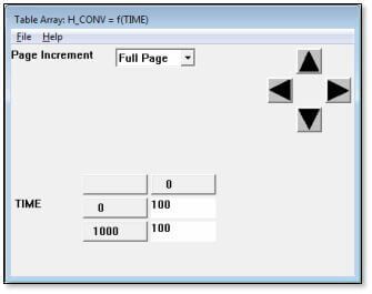
The convection coefficient was applied with the Table Array “H_CONV” which was set to hold a constant value over time, as can be seen below in the figure below:
Element Choice and KEYPOT Settings
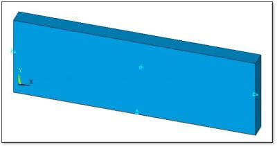
In this example, a solid rectangle has been meshed with a mapped mesh of SOLID226 elements. The SOLID226 element options are shown in the figure below.
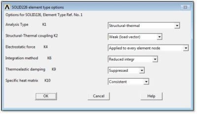
Note the Weak (load vector) coupling (contact not used here), and Reduced Integration settings.
Solution Controls
Large displacement transient analysis has been applied with many substeps. For the purpose of the present test, tightened convergence controls were employed, although such tight settings may not be required in some user models. The model has been simplified by the use of material properties that are not temperature dependent.
It is usually important that the structural analysis transient be suppressed. The following two commands can set the thermal transient analysis ON, and the structural transient analysis OFF in the time integration that is performed in this example:
TIMINT,ON,THERM
TIMINT,OFF,STRUCT
Some of the settings for the current example are shown in the Solution Controls dialog box in the figure below:
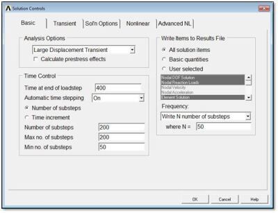
In addition to the above, loading was set to “Ramped” so that the applied non-zero displacement loading in this model is ramped up through the substeps of the load step. Because of the load ramping, the Table Array of the figure above was used to hold constant the convection coefficient load over all substeps.
Outputs from the Example Model
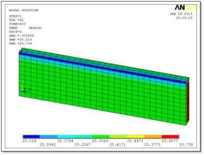
The input material property QRATE for the Taylor-Quinney coefficient was 0.9 in this example, so 90% of the plastic strain energy is converted into heat. The specific heat C and the density DENS are set to values typical of a steel material. One of the available outputs with Ansys materials with kinematic and isotropic hardening is the plastic work per unit volume, PLWK, as plotted for example with PLESOL,NL,PLWK.
A simplified check on a resulting temperature in an adiabatic analysis is to calculate local temperature change with the temperature change calculation:
Delta_T = QRATE*PLWK/C/DENS
Typical values for strains of a few percent in steel produce a temperature change of only a few degrees, which is why this effect is often ignored in structural analysis. More extreme temperature changes may occur during cyclic loading, high-speed metal forming, extrusion, and events better suited to explicit dynamic analysis.
In the present example, the above calculation produced Delta_T of 3.803 degrees. The model started with an initial temperature of 22 degrees, and the resulting peak temperature after a 10% strain was 25.738 degrees—a slightly smaller 3.738 degree temperature change than hand calculated because of convective cooling in the model and because of approximations introduced by element behavior, mesh density and transient integration.
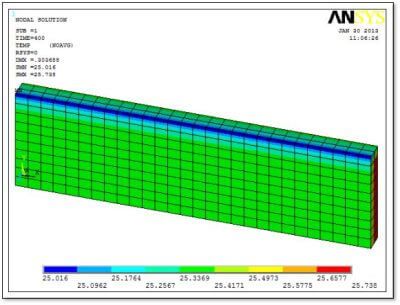
Because the SOLID226 element is a coupled element, deflections, stresses and strains can also be immediately plotted and listed.
A Workbench Mechanical Approach with ACT
Since the early days of Ansys WorkBench Mechanical, it has been possible to insert APDL Command Objects (snippet commands) to modify a structural model. Depending on the location of the snippet commands, one would access different properties of the Finite Element Model and would be able to change it. It was a very efficient way to combine the best of both Mechanical and Mechanical APDL worlds: the power of APDL commands within the user-friendly efficient WorkBench platform. The main drawbacks of this method were that user would have to be very careful with the units, and consistent between the writing of the APDL commands and the definition of the Mechanical model, especially with the Named Selections. To make long story short, it was error prone and not efficient to be deployed across the company.
With R14.5, Ansys has developed the Application Customization Toolkit that enables you to fill the gap between the Mechanical APDL features and their exposure in Mechanical: it is a great improvement that will enable the old snippet commands or old legacy APDL macros to be embedded in custom Mechanical objects that inherits the behavior of standard WorkBench objects. ACT provides you with APIs manipulate a wide range of data (geometry, finite element, material) to change the APDL code which is written when one clicks on the solve button.
![]()
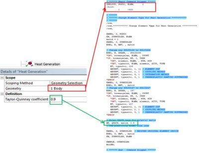
For instance, taking into account heat generation in plastic deformation would require changing the default element type created by the standard interface and adding the desired material property QRATE: it would convert the SOLID186/187 elements into coupled SOLID226/227 elements with the desired keyoptions:
Using Ansys Mechanical APDL and Workbench: Application of the New Act Module
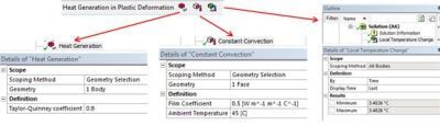
It is assumed that the Engineering Data has supplied all other material properties, including the plasticity model. The figure below includes all the structural and thermal properties that will be needed for the thermoplastic heat generation with the exception of QRATE, which is defined with the ACT objects:
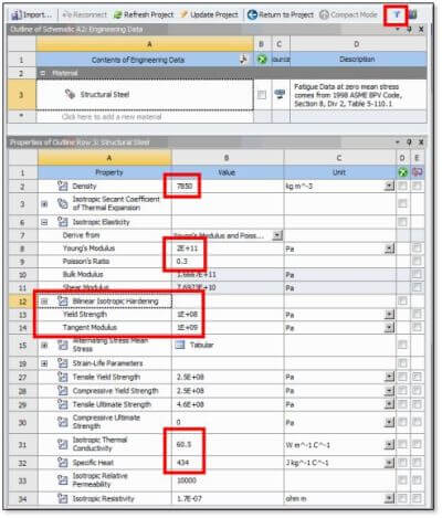
In the figure above, note that the Filter icon has been set so that both thermal and structural properties are available.
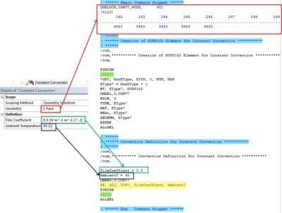
If one would want to add a convection load, a custom constant convection object has been defined: here, no need to take care of the units, Mechanical will handle the conversion on the fly, just like other objects.
The presence of the ‘Heat generation’ object in the tree will also add other commands before the solve in order to convert the Static Structural system into one containing a structural static solution blended with a transient thermal solution:
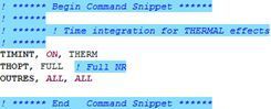
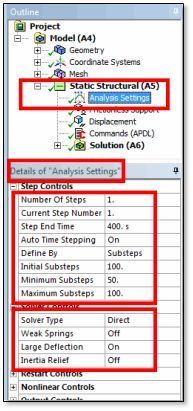
Note the specification of full Newton-Raphson iteration, and the output of all results data, which might be more than the minimum needed. It may be desired to add more convergence tolerance controls. Analysis Settings are set as if a transient analysis takes place, including sufficient substeps and Solver Options, as illustrated in the figure above.
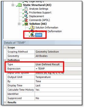
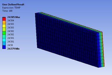
Even thought this is nominally a “Static Structural” system that offers only structural outputs, the temperature result can be plotted in the results section by inserting a User Defined Result, as in the figure below.
A simplified calculation of the temperature change can be implemented the same way it was calculated in Mechanical APDL: it retrieves the correct material properties (QRATE, Specific Heat, Density) and uses the plastic work induced by the deformation, with no input of the user:
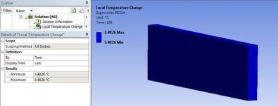
The above calculation can serve as a “sanity check” on results.
Thus, using this extension (new toolbar) we did add some new features to our standard GUI, to better take into account the process we are involved in.
Conclusions | Heat Generation in Plastic Deformation
PLANE223, SOLID226 , and SOLID227 coupled analysis elements permit modeling of thermoplastic heat generation in Ansys models that have nonlinear plastic material properties with the Multiphysics and Mechanical licenses.
Users must be careful to use thermal properties (specific heat and thermal conductivity) expressed in the same units as the energy units of the structural physics in the model. (This means not using BTU in an inches-pounds-seconds system). The simplest choice of a system of units will be SI.
An example model with a steel material resulted in a temperature change of 3.738 degrees when 10% strain was applied. Results depend on yield stress, tangent modulus after yielding, and other details of the material model and post-yield behavior. The example was subject to large-displacement transient simulation with a large number of substeps. Ideal substep size can depend on either the nonlinear structure or the thermal transient details.
These element types have midside nodes and can represent structural deformations in good detail. In some thermal transients the midside nodes mean that users should ensure that time substeps are neither too large nor too small, and that a satisfactory mesh density is employed. Substantial temperature changes can result with extreme plastic deformation—this is sometimes better handled with low-order elements in an explicit dynamic analysis.
Outputs from Ansys can include plastic work per unit volume, so users can calculate approximate expected temperature changes in adiabatic processes directly from the plastic work.
Note that a custom object in an ACT extension can estimate the temperature change caused by plastic work per unit volume, using only a static structural analysis and structural elements, if the temperature changes caused are moderate and do not affect the structure significantly.
With the PLANE223, SOLID226 , and SOLID227 coupled analysis elements, Ansys can address heat generation that results from plastic deformation. User models might blend this effect with other sources of heating, including friction sliding, thermal loads, and electrical effects with Multiphysics modeling.
Because these elements permit direct coupled analysis, nonlinear contact and large displacement effects can directly affect the thermal results, and vice versa. With an ACT extension, Workbench Mechanical can convert a static structural analysis into such a nonlinear coupled analysis with thermoplastic heat generation: