Setting up Thermal Expansion Modeling in Ansys Mechanical Workbench
Materials that undergo extreme thermal expansion when heated are unusual, but occasionally users may want to model extreme swelling of a body or capture another effect by using thermal expansion to increase the size of elements. The present example examines what happens in Ansys when an extreme coefficient of thermal expansion is employed. Ordinary coefficients of thermal expansion are on the order of 1.0e-5 or 1.0e-6. The present example uses a coefficient of 0.01 over a range of 100 degrees C.
Two concerns are examined: (1) During large displacement analysis, solution substeps employ an updated thermally expanded size of elements to calculate thermal expansion during each next substep. (2) The model tested whether mass increases as element size grows, and whether a temperature-dependent mass density must be entered.
Time-Varying Temperature Load in Ansys Mechanical Workbench
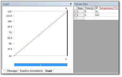
Ansys Mechanical can ramp up applied temperatures during substeps in a structural model. These temperatures affect temperature-dependent material properties, and cause thermal expansion. Temperatures might be imported from a thermal analysis, or might be applied directly in a structural simulation. In the present example, a uniform temperature is applied to a selected body. The temperature is ramped up over time, starting at the ambient value of 22C, and rising to 122C, for a 100C increase.
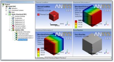
The Thermal Expansion Structural Model
A simple Ansys structural model of a 1-meter cube is map meshed with low-order (no midside nodes) elements.
Displacement constraints are applied perpendicular to 3 faces. One prevents UX, one prevents UY and one prevents UZ.
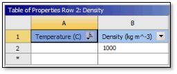
A constant (not ramped) gravity load is applied as an Acceleration object. It is set to 9806.1 mm/sec^3 in the Y direction. The material density is set to 1000 kg/m^3, so the vertical reaction force should be a constant 9806.1N in the Y direction throughout the analysis.
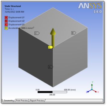
A time-dependent thermal load is applied to the body. As shown above in the second figure, temperature is ramped from ambient 22 degrees C up to 122 degrees C. Analysis settings were set to ramp up the load through 100 substeps. This is done in order to integrate the increasing thermal expansion with accuracy.
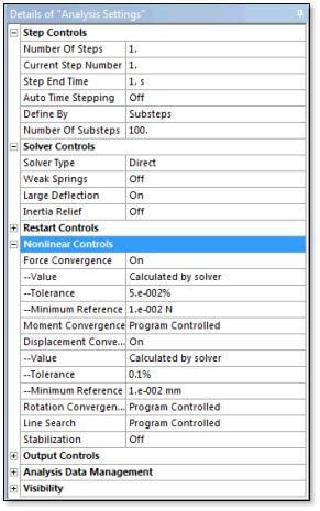
Solver Controls set Solver Type to Direct, because of the small size of the model.
Weak Springs are Off, and Large Deflection is ON. Because of the large amount thermal expansion, loads due to weak springs were not wanted, and there are enough displacement constraints (supports) to prevent free rigid body motion, so the weak springs are unnecessary.
Nonlinear Controls are set to a tighter-than-default value to get an accurate value of reaction force, and insight as to how the mass matrix is treated during extreme thermal expansion.
Displacement Convergence is added to ensure that thermal expansions that cause little force buildup will be captured in addition to the reaction forces.
Coefficient of Thermal Expansion
If a small displacement analysis is performed, applying an Isotropic Secant Coefficient of Thermal Expansion is quite simple. Values that may be temperature-dependent are entered as Engineering Data in the Ansys Workbench interface. No integration over intermediate temperatures is required for thermal expansion to reach a correct value, even when the coefficients are temperature dependent, because the secant value is employed.
With large displacement analysis, thermal expansion is treated in a more complex manner. At any particular substep or load step, an increment of thermal expansion is based on an increment of temperature change, and the current dimensions of each element. This effect is not noticed with thermal expansion coefficients on the order of 1.0e-5, but becomes evident with values of 1.0e-2 or 1.0e-3.
Knowing that the thermal expansion will be integrated over substeps and that the temperature is ramping up during the substeps, values entered for thermal expansion coefficients can be adjusted accordingly. The shortcoming of compensating for nonlinear large displacement in this manner is that only one “real” coefficient of thermal expansion can be represented—it is not temperature dependent. The desired coefficient of thermal expansion can be adjusted in this manner:
αT = ln(α×(T-TREF)+1)/(T-TREF)
where
αT = Coefficient of Thermal Expansion to use in Large Displacement analysis.
T = Temperature for an αT value
α = Coefficient of thermal expansion desired in resulting analysis, NOT temperature dependent.
TREF = Reference temperature for thermal expansion, usually 22C
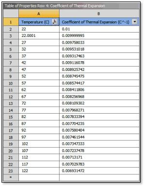
The αT values are entered into Engineering Data as “Isotropic Secant Coefficient of Thermal Expansion” in Tabular format as a function of T. When a large displacement analysis is performed, the “real” thermal expansion based on the desired coefficient α will be obtained.
The figure below shows a table of thermal expansion coefficients to use in an extreme thermal expansion example. Reference temperature is 22C. It is desired to achieve a coefficient of thermal expansion of α = 0.01. The values shown in Figure 5 will result in thermal expansion based on 0.01 when large displacement nonlinear analysis is employed as illustrated in Figure 4, and the applied temperature 122C is ramped up from TREF through substeps. Since the temperature change is 100C, and α = 0.01, then a doubling of each linear dimension is expected. Note the use of a dense set of temperatures in the Temperature column, for accuracy.
Mass Density | Non-Temperature Dependent in Thermal Expansion
Testing with Ansys Mechanical showed that the mass density does NOT need to be adjusted according to the temperature of the amount of thermal expansion. With a single mass density entered (not temperature dependent), the reaction force was constant throughout the analysis (within convergence tolerance) when a constant gravity load was applied and temperatures were ramped up over substeps.
Evidently Ansys does not consider the net mass of an element to need to be adjusted as a result of volume changes.
Analysis | Thermal Conditioning on Convergence Tolerance
A Thermal Condition is ramped up through substeps as shown in Figure 2: Thermal Condition on a Selected Body and Figure 4: Analysis Settings. The resulting thermal expansion doubled each of the three linear dimensions of the cube. The vertical force reaction was constant within the convergence tolerance, with the mass density held constant and not a function of temperature.
Because in large displacement analysis, thermal expansion is based on the current size of the model from one substep to the next, the object will expand exponentially, unless the effect is undone when the coefficient of thermal expansion is modified with the equation αT = ln(α×(T-TREF)+1)/(T-TREF). This is easily implemented in a spreadsheet calculation. As noted, the consequence is that only one “real” coefficient of thermal expansion α can be represented, and it is not temperature dependent.
Postprocessing of Thermal Expansions
Thermal expansions can be plotted after the solution completes successfully:
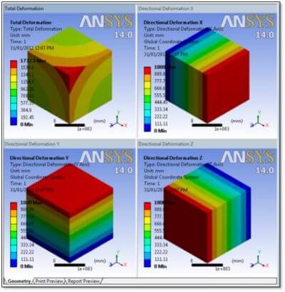
Animations can show the history. Users may choose to create the animations at a reasonably large number of equally spaced points in time (linear interpolation for values is used), or only at the time points recorded in the results file.
![]()
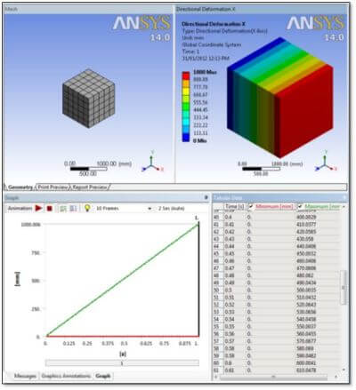
The following figure shows thermal expansion in the X direction. The X dimension has doubled, as desired, since a temperature increase of 100C has been applied with a “real” coefficient of thermal expansion of α = 0.01. Of interest is that the growth at time=0.5, when the temperature would have increased by 50C, is 500mm (within a tolerance), illustrating that the approach works over a variety of temperatures.
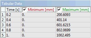
If the number of substeps is reduced, the analysis completes more quickly, but the accuracy of the thermal growth calculation is reduced. This is illustrated by the above analysis performed over only 5 substeps:
Summary | Extreme Thermal Expansion Modeling in Ansys Workbench
This article has described a means of including extreme thermal expansion in an Ansys Mechanical Workbench Finite Element Analysis. If substantial swelling of a model is to be modeled via large coefficients of thermal expansion, testing illustrates that a non-temperature-dependent coefficient of thermal expansion α can be made to work “properly” if an Engineering Data table of coefficients of thermal expansion is entered for a dense set of temperatures with the α value adjusted at each temperature T by the formula:
αT = ln(α×(T-TREF)+1)/(T-TREF)
The procedure lets a large displacement solution with a sufficient number of substeps during any thermal ramped load predict thermal growths that results in substantial increases in the linear dimensions and volume of a body. Testing with a Workbench model illustrated that the mass density does not have to be adjusted as a function of temperature when volume changes result during an analysis.
Accuracy in the predicted results requires a reasonably large number of substeps in order to numerically integrate the thermal expansion over a temperature range, and tight tolerances on nonlinear force and deflection results. “Soft springs” should be turned off in Workbench Mechanical, and “Large Displacement” turned on. Sensitivity tests should be employed to illustrate that solutions are accurate, varying the number of substeps, using a generous number of αT entries over the temperature range, and employing tight nonlinear tolerance.
With small coefficients of thermal expansion, such as 1.0e-5, the αT formula above is not required when large displacement nonlinear analysis takes place, and the “real” temperature-dependent coefficients of thermal expansion can be employed as desired.
Testing suggests that mass density does not need to be adjusted as a function of thermal expansion, even if substantial changes in element volume will result during the analysis.
Using the method illustrated in this document should permit a user to implement substantial growth in the volume of elements or bodies, as driven by temperature changes, in order to creatively capture a variety of “swelling” or other effects in FEA modeling.