How do I Linearize Stress in Ansys Mechanical?
Ansys Workbench Mechanical can use the Construction Geometry branch of its Outline to define planes in space onto which User Defined Results from selected geometry can be mapped from selected bodies. Although some math can be done on these results, the range of operations required to perform linearization of stress distributions is more complex, and can be aided by APDL Commands Objects.
This article illustrates an approach to using APDL Commands Object to map and linearize results on a plane.
Setup Ansys Workbench Mechanical Construction Geometry
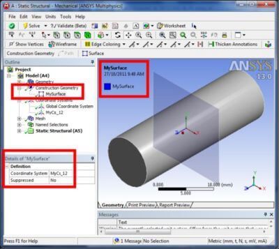
In a Workbench Mechanical model, a Construction Geometry can be inserted in the Model Outline, and used to define a surface that cuts across the interior of a 3D solid model. In the image below, a surface called “MySurface” has been defined to be on the X-Y plane of the user-defined Coordinate System “MyCs_12”. The surface can be seen to cut through the interior of a solid model of a cylinder.
The user-defined coordinate system will be employed in the Ansys macro that follows. Defining the section for plotting purposes is used to check positioning of the cutting plane and provides a plot useful in a report, but only the user-defined coordinate system is used in the macro.
The coordinate system used above to position the surface is called “MyCS_12” and can be defined in various ways. In the following figure, it is positioned from existing geometry. In this example, the X and Y axis directions are related to the Global Cartesian axes.
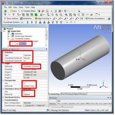
Note in the figure above that a Manual setting of Coordinate System ID has been employed. In this example it was set to “12”, which was also used in the name of the coordinate system “MyCS_12” for ease of identification. This coordinate system number will be used later in work done by the inserted APDL Commands Object to position a Working Plane that cuts through the elements of chosen geometry. The coordinate system number “12” can be passed as an argument to the APDL Commands Object, as illustrated further below.
A Named Selection will be used to indicate which bodies are to be sliced by a surface for mapping and linearization for a Commands Object. Multiple versions of the Commands Object can be inserted in the Outline at the post-processing stage below Solution to evaluate different surfaces that cut through 3D solid models in various locations. Each can be provided with a different Named Selection to indicate the body or bodies that are to be cut. The component that is the Named Selection will have to be entered directly into an individual APDL Commands Object.
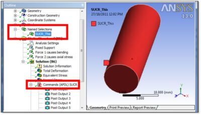
In the above figure, a Named Selection “SUCR_This” identifies a body that is to be sliced by a cutting plane with the surface mapping of stresses to be mapped in an APDL Commands Object that is inserted in the postprocessing Solution branch of the Outline. The Named Selection solid body will be selected inside the Commands Object with a CMSEL command. The slice is indicated by reference to the coordinate system number “12” applied manually to the coordinate system named “MyCS_12” above. Only the number “12” is relevant in defining the coordinate system in the example presented here:
My_Cs=ARG1 ! specify the coordinate system, ARG1 of macro call
cmsel,s,SUCR_This ! select elements of body/bodies of interest
nsle ! select their nodes
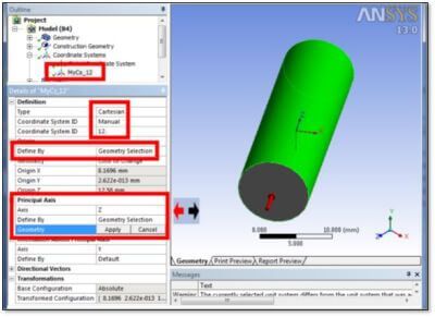
The surface onto which stresses will be mapped for linearization will typically be perpendicular to a major axis on a body. In a second example in the figure below, the geometry of a body is used to align and orient the surface by positioning the Z-axis of the local coordinate system used to define the surface. I this second example, the body’s major axis is not aligned with the Global Cartesian axes:
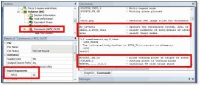
Note in the following figure that the ARG1 argument “12” is used to define the position of the working plane, and that the elements of the Named Selection “SUCR_This” are selected for the surface results mapping that follows:
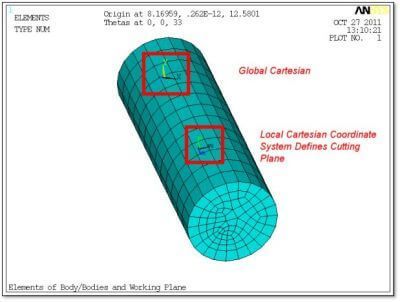
The following figure shows the mesh within the Ansys Batch job, and two coordinate systems: the Global Cartesian system, and Local Coordinate System “12” as defined in the Workbench Mechanical Outline. System “12” will be used to position the cutting plane for stress linearization.
The APDL Commands Object macro presented in this document is used to linearize bending stress on a cross-section. It does not consider what to do with shear and torsional loads on the section cut through the selected body. Such an “exercise for the reader” should consider both: (1) whether a linearized shear or torsional load significant in overloading a part at the cutting plane, and (2) whether design codes, contracts, or product safety considerations that are to be satisfied require such loads to be evaluated in a linearized fashion.
Map Stress onto Cutting Plane & Linearize for Average Stress Perpendicular
The following figure is the content of the APDL Commands Object that will map stresses onto the cutting plane, linearize those stresses for average stress perpendicular to the cutting plane, and bending stress about the centroid of the cut section, add the normal and linearized bending stress, and plot results. The content of the Commands Object will need to have the Component name (from the Named Selection for the body of interest) and the coordinate system number changed for each surface to be postprocessed for linearization.
Figure below: APDL Commands Object Listing to Linearize Stress on a Surface
! Position working plane at triad of specified coordinate system.
! Z axis of working plane should be perpendicular to cut across 3D body/bodies of interest.
!
! Calculate Mx, My about center of surface on working plane.
! Map linearized Mc/I onto the surface.
!
! It is important that the WP is located on the axis of interest
! for the purpose of shear, torsion, and hoop stress work.
!
! SUCR stores the following quantities for the defined surface:
! — GCX, GCY, GCZ are global Cartesian coordinates at each
! point on the surface.
! — NORMX, NORMY, NORMZ are components of the unit normal at each
! point on the surface.
! — DA is the contributory area of each point.
!
! Call after placing Coordinate System where it cuts the model at position of interest.
! Cut will be across the elements of the body in the Named Selection “SUCR_This”
!
!
! At this point we are in /POST1
!
/com, .
set,last ! read in result of last load step/substep <<===== #####
/com, .
!
! Plan PNG image files
!
pngr,comp,on,9 ! compression
pngr,orient,horizontal ! orientation
pngr,color,2 ! color versus B&W or grey
pngr,tmod,1 ! bitmap text
/gfile,600 ! Or, use 967 –> 0.75 * (6.5 x 200 – 10) pixels, 6.5″ wide 200 DPI lscape
/RGB,INDEX,100,100,100, 0 ! black/white reversal
/RGB,INDEX, 80, 80, 80,13
/RGB,INDEX, 60, 60, 60,14
/RGB,INDEX, 0, 0, 0,15
/COLOR,PBAK,OFF ! clear background
!
/PLOTPS,INFO,3 ! Multi-legend mode
/PLOPTS,WP,ON ! Working plane plotted
!
!
/show,png ! Generate PNG image files for Workbench
!
My_Cs=ARG1 ! specify the coordinate system, ARG1 of macro call
cmsel,s,SUCR_This ! select elements of body/bodies of interest
nsle ! select their nodes
*get,numelements,elem,,count ! how many elements in the body/bodies
*if,numelements,eq,0,then
*MSG,ERROR
The indicated body/bodies in SUCR_This contain no elements
/EOF
*endif
!
WPCSYS,,My_Cs ! place working plane at origin of coord sys ARG1
/CPLANE,1 ! cutting plane is working plane
WPSTYL,,,,,,0,2,1 ! cartesian WP with triad shown
!
! Check existence of coordinate system in ARG1
*GET,csexist,CDSY,My_Cs,ATTR,KCS
*if,csexist,GT,-1,then
! perform calculations
/com, .
/com, .
/com, Checking origin and orientation of “My_Cs” coord sys
/com, .
*GET,x_orig,CDSY,My_Cs,LOC,X ! find the origin
*GET,y_orig,CDSY,My_Cs,LOC,Y
*GET,z_orig,CDSY,My_Cs,LOC,Z
*GET,THXY,CDSY,My_Cs,ANG,XY ! find the orientation
*GET,THYZ,CDSY,My_Cs,ANG,YZ
*GET,THZX,CDSY,My_Cs,ANG,ZX
/annot,dele ! delete existing annotations if any
/VIEW,1,1,2,3
/ANG,1
/ANNOT,DELE
/ANUM ,0, 1, -0.32, 0.92000
/TLAB,-0.32, 0.92,Origin at %x_orig%, %y_orig%, %z_orig%
/ANUM ,0, 1, -0.32, 0.86000
/TLAB,-0.32, 0.86,Thetas at %THXY%, %THYZ%, %THZX%
/title,Elements of Body/Bodies and Working Plane
eplo
/title,Nodes of Body/Bodies and Working Plane
nplo
! /ui,copy,save,png,graph,color,norm,portrait,yes
/com, .
/com, .
/com, The SUCR command to create “mysurf” ##############
/com, Surface is defined by the cutting plane in window 1 (controlled by working plane (/CPLANE,1)
!
SUCR,mysurf,CPLANE,2 ! form the surface on Working Plane, accuracy 2. Automatically creates:
! GCX, GCY, GCZ – global Cartesian coord at each point on the surface.
! NORMX, NORMY, NORMZ – components of the unit normal at each point on surf.
! DA – the contributory area of each point
!
SUSEL,S,mysurf ! select this surface; it is used below
/title,Plot coordinates on working plane cut prior to transformation
SUPL,mysurf,GCX
SUPL,mysurf,GCY
SUPL,mysurf,GCZ
!
/annot,dele
!
! Will tranform X, Y, and Z coord of mapped surface so that data exists in Working Plane X,Y
!
! Note: The following *GET commands return rotations in DEGREES for the working plane position
!
*get,thxy,CDSY,4,ANG,XY ! First rotation, about the Global Z axis, that put working plane where it is
*get,thyz,CDSY,4,ANG,YZ ! Second rotation, abou the new X axis, that put working plane where it is
*get,thzx,CDSY,4,ANG,ZX ! Third rotation, about the newest Y axis, that put working plane where it is
!
*get,origx,CDSY,4,LOC,X ! location of the origin of the working plane, in Global Cartesian
*get,origy,CDSY,4,LOC,Y ! location of the origin of the working plane, in Global Cartesian
*get,origz,CDSY,4,LOC,Z ! location of the origin of the working plane, in Global Cartesian
!
! Form cosine and sin terms as used in a rotation matrix
/com, .
/com, .
/com, Form cosine and sin terms as used in a rotation matrix
!
*afun,deg ! treat theta values as degrees
c1=cos(thxy) ! Cosine of THXY, first rotation about Global Z
s1=sin(thxy)
c2=cos(thyz) ! Cosine of THYZ, second rotation about the new X
s2=sin(thyz)
c3=cos(thzx) ! Cosine of THZX, third rotation about the newest Y
s3=sin(thzx)
*afun,rad ! return to default radians
!
! Form terms needed in first 2 rows of the 3×3 rotation matrix
R11=c3*c1-s3*s2*s1
R12=c3*s1+s3*s2*c1
R13=-s3*c2
R21=-c2*s1
R22=c2*c1
R23=s2
!
! Terms of the third row if wanted for checking purposes
! R31=s3*c1+c3*s2*s1
! R32=s3*s1-c3*s2*c1
! R33=c3*c2
!
! Create data that results if the average X, Y, Z in global coord are translated back to global origin
!
! Employ these rotation terms to create Surface Operations results data containing
! the X and Y values of surface data as would be measured in the working plane.
! Global Coordinates of points on the surface before transformation are GCX, GCY, and GCZ
! Place the above terms as surface data for subsequent SUCALC operations
!
! Note: DA acts as a dummy in the following:
!
/com, .
/com, .
/com, Placing zeros on the surface for various items #############
! Form a ZERO on the surface
SUCALC,MyZero,DA,ZERO,,,,0.0
!
! Form R11 values etc over the surface (EVERY POINT ON SURFACE GETS THE VALUE):
!
SUCALC,sr11,DA,ZERO,,,,r11 ! rotation matrix terms
SUCALC,sr12,DA,ZERO,,,,r12
SUCALC,sr13,DA,ZERO,,,,r13
SUCALC,sr21,DA,ZERO,,,,r21
SUCALC,sr22,DA,ZERO,,,,r22
SUCALC,sr23,DA,ZERO,,,,r23
!
! SUCALC,sr31,DA,ZERO,,,,r31 ! third rotation data if wanted
! SUCALC,sr32,DA,ZERO,,,,r32
! SUCALC,sr33,DA,ZERO,,,,r33
!
/com, .
/com, .
/com, Forming working plane coord from CGX, GCY, GCZ and rotation
! Form working plane coordinates by multiplying matrix rows by vector of GCX, GXY, GCZ
! First do X
SUCALC,WPX1,sr11,MULT,GCX ! R11*X
SUCALC,WPX2,sr12,MULT,GCY ! R12*Y
SUCALC,WPX3,sr13,MULT,GCZ ! R13*Z
SUCALC,WPX,WPX1,ADD,WPX2
SUCALC,WPX,WPX,ADD,WPX3 ! Form X ON WORKING PLANE = R11*X+R12*Y+R13*Z
!
! Then do Y
SUCALC,WPY1,sr21,MULT,GCX ! R21*X
SUCALC,WPY2,sr22,MULT,GCY ! R22*Y
SUCALC,WPY3,sr23,MULT,GCZ ! R23*Z
SUCALC,WPY,WPY1,ADD,WPY2
SUCALC,WPY,WPY,ADD,WPY3 ! Form Y ON WORKING PLANE = R21*X+R22*Y+R23*Z
!
! Z for checking — all points should be on the same plane
! SUCALC,WPZ1,sr31,MULT,GCX ! R31*X
! SUCALC,WPZ2,sr32,MULT,GCY ! R32*Y
! SUCALC,WPZ3,sr33,MULT,GCZ ! R33*Z
! SUCALC,WPZ,WPZ1,ADD,WPZ2
! SUCALC,WPZ,WPZ,ADD,WPZ3 ! Form Z ON WORKING PLANE = R31*X+R32*Y+R33*Z
!
! Find average X, Y, and Z values on the plane for the WPX, WPY, WPZ data
!
/com, .
/com, .
/com, Finding average X, Y, Z on plane from working plane coord
SUEVAL,avg_x,WPX,AVG
SUEVAL,avg_y,WPY,AVG
! SUEVAL,avg_z,WPZ,AVG
!
! We do not always have a perfect circle so get X and Y relative to average
! Find X, Y, Z of points on surface relative to the average point
! Calculate the local X, Y, Z of points on the surface
/com, .
/com, .
/com, Subtracting average X, Y, Z from the working plane X, Y, and Z coord
SUCALC,LCX,WPX,SUB,MyZero, , ,-avg_x ! X coord measured from avg_x
SUCALC,LCY,WPY,SUB,MyZero, , ,-avg_y ! Y
! SUCALC,LCZ,WPZ,SUB,MyZero, , ,-avg_z ! Z
!
/com, .
/com, .
/com, Plot transformed coordinates on the working plane cut
/title,Plot coordinates on working plane cut AFTER transformation
SUPL,mysurf,LCX
SUPL,mysurf,LCY
! SUPL,mysurf,LCZ
!
/com, .
/com, .
/com,Forming squares of X and Y measurements
! Find squares of the local X and Y measurements
SUCALC,LCXsq,LCX,MULT,LCX, , ,0, ! X coord measured from avg_x
SUCALC,LCYsq,LCY,MULT,LCY, , ,0, ! Y
!
/com, .
/com, .
/com, Integrating to get Ixx and Iyy
! Integrate to get Ixx and Iyy
SUEVAL,Ixx,LCYsq,INTG ! Ixx (about avg_x)
SUEVAL,Iyy,LCXsq,INTG ! Iyy (about avg_y)
!
*get,max_cs,CDSY,,NUM,MAX ! maximum coordinate system number
!
*if,max_cs,le,10,then ! set to 10 if necessary so that next CS is 11.
max_cs=10
*endif
!
/com, .
/com, .
/com, Creating local cartesian CS on the working plane
CSWPLA,max_cs+1,0 ! align local CS Cartesian on WP, becomes active CSYS
RSYS,max_cs+1 ! use this local coordinate system
!
/com, .
/com, .
/com, Mapping SZ onto the surface
! Give the user something to look at
SUMAP,sax,S,Z ! map Sz (axial) onto the surface. AXIAL STRESS <<===
/com, .
/com, .
/com, Plotting SZ as mapped onto the surface
/title,SZ Mapped onto the surface
SUPL,MYSURF,sax,1 ! plot the mapped result with element edges
!
/com, .
/com, .
/com, Form results in a cylindrical coordinate system
!
CSWPLA,max_cs+1,1 ! switch to a cylindrical system
RSYS,max_cs+1 ! use this local coordinate system
SUMAP,s_thetaz,s,yz ! torsional stress (y=theta, z=axis)
SUMAP,s_hoop,s,y ! hoop stress (y=theta)
!
CSWPLA,max_cs+1,0 ! back to cartesian system
RSYS,0 ! back to Global Cartesian results
!
/com, .
/com, .
/com, Form products of axial stress with Local X and Y
sucalc,sax_y,sax,MULT,LCY ! Used below to calculate Mx
sucalc,sax_x,sax,MULT,LCX ! Used below to calculate My
!
/com, .
/com, .
/com, Form integrals. This produces moments about the origin.
sueval,Mx,sax_y,INTG
sueval,MY_neg,sax_x,INTG ! This is the negative of My
!
/com, .
/com, .
/com, Calculate averaged values of hoop stress and torsional stress
SUEVAL,avg_hoop,S_HOOP,AVG
SUEVAL,avg_theta,S_THETAZ,AVG
!
/com, .
/com, .
/com, Calculate averaged value of direct axial stress
SUEVAL,avg_axial,sax,AVG
/com, .
/com, .
/com, Net Moment
M_net=sqrt(Mx**2+My_neg**2)
!
/com, .
/com, .
/com, Form M/I values for user in Mc/I further below
Mx_Ixx=Mx/Ixx
My_Iyy=-My_neg/Iyy
!
/com, .
/com, .
/com, Place these M/I values on surface prior to calculation of Mc/I values
SUCALC,MxIxx,DA,ZERO,,,,Mx_Ixx
SUCALC,MyIyy,DA,ZERO,,,,My_Iyy
!
/com, .
/com, .
/com, Form Mc/I values–note term with minus sign.
! Step 1: Sz due to Mx (term gets plus sign in summation further below)
SUCALC,sz_mx,LCY,MULT,MxIxx
! Step 2: Sz due to My (term gets minus sign in summation further below)
SUCALC,sz_my_neg,LCX,MULT,MyIyy
!
/com, .
/com, .
/com, Form sums of stresses
SUCALC,sz_lin,sz_mx,SUB,sz_my_neg ! combine the two axial stresses due to bending
!
/com, .
/com, .
/com, Form average axial stress (one value)
SUCALC,sz_axavg,DA,ZERO,,,,avg_axial
!
/com, .
/com, .
/com, Form sum of average axial stress (constant) and linearized bending stress
SUCALC,sz_lin2,sz_lin,ADD,sz_axavg
/com, .
/com, .
/com, Linearized stresses (membrane plus/minus bending) on the cut
/title,Linearized Stress on the Cut, Due to Bending Only
/ANNOT,DELE
/ANUM ,0, 1, -0.32, 0.92000
/TLAB,-0.32, 0.92,Mx=%Mx%, My=-%My_neg%
/ANUM ,0, 1, -0.32, 0.86000
/TLAB,-0.32, 0.86,M_net=%M_net%
!
SUPL,MYSURF,sz_lin,0 ! without element edges
SUPL,MYSURF,sz_lin,1 ! with element edges
!
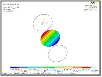
/title,Linearized Bending+Axial Stress Normal to Cut, No Torsion or Shear.
/ANNOT,DELE
!
SUPL,MYSURF,sz_lin2,0 ! without element edges
SUPL,MYSURF,sz_lin2,1 ! with element edges
!
*else
/com, .
/com, .
/com, Coordinate system requested in ARG1 does not exist
*MSG,WARN,My_Cs
Coordinate system %G% in argument to this macro does not exist.
!
*endif
!
! Exit here
/title
rsys,0
csys,0
allsel
There is some unnecessary content in the above APDL code, including various comments that indicate where the commands have executed in the Output file that is generated by the Ansys Batch job, and some unnecessary extra coordinate system work and measurements of coordinate system orientations.
Employ Ansys APDL Commands to Process Shear, Torsional Stresses and Bending Stresses
The plots generated in this APDL code explore some output possibilities. Users may wish to orient the viewing direction for the plots, by adjusting the arguments to the /VIEW command. These arguments could be based on the orientation angles measured for the coordinate system that defines the cutting plane, or otherwise determined by a user’s commands.
Users may also wish to add some commands that process shear and torsional stresses, and consider adding their effects to the linearized average and bending stresses on the cutting section.
A brief summary of the steps required for this stress linearization on cutting planes is:
- Select a body of interest and refer to it in a Named Selection.
- Define a Cartesian coordinate system that cuts the body. Record the coordinate system number.
- Place the APDL macro in a postprocessing Commands Object. Provide an argument with the coordinate system number, and change the name in the Component selection to the one in the Named Selection.
- Do the above for each body of interest.
- Solve the model, and look at the postprocessing results.
Sample Results | “Scoping Method” for Linearized Stress
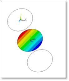
The following plot shows stress normal to a surface. It is generated by referring to Surface as a “Scoping Method”, choosing the surface from a drop-down list, and filling in the Definition to indicate “Orientation” and the “Coordinate System” for the result of interest. It does not show a linearized stress.
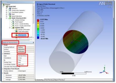
Note that in the Details section, numerical Results output includes an Average value for the normal stress. What is missing is a reference to linearized bending, and the sum of linearized bending stress and average normal stress.
Stresses are mapped onto the locations where the cutting plane goes through the 3D elements of the selected geometry by the macro. Integrations and other operations are performed on the data that is mapped to the surface, resulting in linearized membrane average and linearized bending results.
The math operations employed in the presented macro are taken from the Surface Operation commands available in Ansys. For reference, some of the following commands are employed in the macro example:
Surface Operations Commands
These /POST1 commands are used to define an arbitrary surface and to develop results information for that surface:
SUCALC Create new result data by operating on two existing result datasets on a given surface.
SUCR Create a surface.
SUDEL Delete geometry information as well as any mapped results for specified surface or for all selected surfaces.
SUEVAL Perform operations on a mapped item and store result in a scalar parameter.
SUGET Create and dimension an NPT row array parameter named PARM, where NPT is the number of geometry points in SurfName.
SUMAP Map results onto selected surface(s).
SUPL Plot specified SetName result data on all selected surfaces or on the specified surface.
SUPR Print surface information.
SURESU Resume surface definitions from a specified file.
SUSAVE Save surface definitions and result items to a file.
SUSEL Selects a subset of surfaces.
SUVECT Operate between two mapped result vectors.
Summary | Linearizing Stress Distribution in Ansys Mechanical
A macro has been employed in a Workbench Mechanical postprocessing APDL Commands Object to form linearized membrane average and linearized bending stress on a plane section that cuts across a body in the model. Surface Operations are used to carry out the mapping, multiplications, integrations and summations required on the surface to form these postprocessing results. An example use of the macro has been illustrated in a simple model.
Much of the correct use of this macro will result from user settings. The location of the cutting plane must be indicated with a local coordinate system with the coordinate system number applied manually by the user. A Construction Geometry “Surface” can be entered to make the location of the section more visible to the user, and in a report, but is not a necessity in employing the macro.
The user must select the solid geometry that is to be cut by the surface section, and supply it to the macro as a Named Selection. Elements of that Named Selection are selected as a Component inside the APDL commands.
The current example of the macro returns membrane average stress that is normal to the section cut through the body, and a linearized bending result. The contributions of these two results are summed and the result is plotted.
The user must determine how to orient the cutting plane—the present macro is just one example. This would become challenging in a model with large rotations in the body or bodies of interest.
The user must decide how to apply linearized stress values in assessment of a structure, and in satisfaction of the requirements of a design code. The user must also decide how to approach assessment of any torsional or shear effects at the cutting plane, particularly when warping can result. Material behaviors are assumed linear. A user must decide how to assess structures with material yielding or other nonlinear effects.
Ansys also has Path linearization techniques that assess linearized results along a line through a section. The present area-based technique is a newer possibility, and does not necessarily satisfy existing design codes.
Contact for Additional Ansys Mechanical and/or Stress Linearization Command Support
Finally, we hope that you can make productive use of our Stress Linearization Commands rundown to enhance your Ansys Workbench Mechanical models. For more information, or to request engineering expertise for a particular use-case scenario surrounding Stress Linearization of Geometric Optimization Techniques, please contact us here.